SINGLE-PHASE HYDRAULICS, SYNERGI PIPELINE SIMULATOR (SPS)
Piping and pipeline design engineers are familiar with the dangers of pressure surges (commonly referred to as “water hammer”) in liquid-filled pipes/pipelines. Pressure surges can be caused by transient events, such as valve closures and pump trips, that cause a pressure wave to move through the piping system at a high speed. The magnitude and speed of the pressure wave are determined primarily by the nature of the transient event (for instance, how fast the valve closes) and the speed of sound of the fluid, but also depend on the pipe material, diameter, wall thickness, and conditions of whether/how the pipe is constrained from moving. Pressure surges can burst the pipe or produce a vacuum, which may lead to collapse of the pipe.
A problem associated with pressure surges, transient piping loads, is also important, but less well understood by most engineers. This discussion examines the fundamentals of transient piping load analysis, the tools that are used to perform the analysis, and how evoleap can add value with this type of analysis.
Consider pipe segment that contains a straight horizontal section, with two vertical sections; each with a 90° bend connecting the vertical sections to the horizontal section as shown in Figure 1. The fluid exerts four forces on the pipe: gravity, friction, the downstream pressure force (F2), and upstream pressure force (F1). At steady-state conditions the pipe is static, so the sum of the forces in the horizontal and vertical directions must be zero. In the horizontal direction the friction force (Ffric) balances the difference in the pressure forces (F1 and F2). In the vertical direction the gravitational force (Fgrav) is balanced by upward forces exerted by pipe supports and/or the pipe segments at the bends.
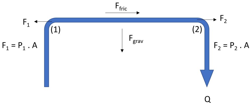
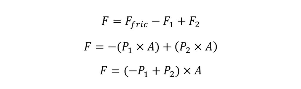
In almost all cases, the frictional force, as we will show, is small and can be ignored. Also, the gravity force, provided the pipe remains full of liquid, is effectively constant, so it is irrelevant to a transient analysis. The pressure forces are equal to the product of the pressure at the specified location and the inner pipe wall surface area. With 90° bends, the direction of the force is along the pipe axis of the pipe segment. The sum of the forces in the horizontal direction is given in the equations below.
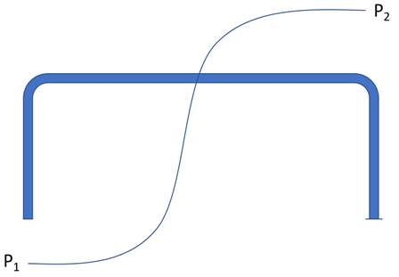
When a valve is closed downstream of the segment, the behavior is different. The valve closure will generate a pressure surge that will propagate backwards through the piping system. At some point, shortly after the valve is fully closed, the pressure wave will reach the pipe segment of interest as illustrated in Figure 2. At that time, the pressure at the downstream bend is much greater than the pressure at the upstream end, resulting in a large, net force in the direction of flow, which can cause damage to the pipe and/or supports or cause the pipe to jump off its supports. For a long pipe segment (~1000 ft), the pressure wave will traverse the entire segment in roughly 0.3 s.
Synergi Pipeline Simulator (SPS) is the industry-leading, transient, single-phase, pipeline simulator and is well-suited for this type of problem. In plants and terminals there are hundreds or thousands of pipe segments. Calculating and extracting the piping loads for different transient cases is a tedious, but important task. This has led evoleap to develop automated techniques for setting up, calculating, and extracting the piping loads from transient simulations for complex piping systems.
The piping load calculations are done via SPS’s application development language, intran, using macros. Macros can be thought of as subroutines that are invoked via a single statement that passes the necessary arguments. Thus, one macro can be used to calculate all the pipe forces where the macro is invoked for each pipe segment. The code to invoke the macros is generated automatically using Excel. SPS calculates the piping load for each segment at every time step in the simulation. The results, piping loads as a function of time and extreme piping loads, are extracted and analyzed automatically with evoleap’s inhouse tools.
We take as an example, the flow of Liquified Natural Gas (LNG) through a 30”, horizontal pipe segment 790 ft long, bounded by 90° bends upstream and downstream initially flowing at a standard loading/unloading rate for LNG. These are typical pipe sizes and segment lengths for LNG loading and receiving terminals. LNG loading and unloading terminals must be particularly cognizant of pressure surges and the resulting piping loads because they operate at high flow velocities, typically at 15 ft/s or greater and have fast valve closures during Emergency Shutdowns (ESDs).
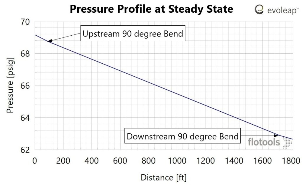
The pressure profile at steady state through the pipe segment is shown in Figure 3 where the left axis (~80 ft) is at the upstream 90° bend. The downstream 90° bend is at the right axis at ~870 ft. Since the pipe is horizontal the difference in pressure across the pipe segment is accounted for entirely by friction. The pressure drop is only 2.9 psi, so the frictional force is obviously small. For instance, the force on each end is P*A = 68.8 psi * 672 in2 = 46.2 kips whereas the frictional force is (P2 – P1) * A = 2.9 psi * 672 in2 = 1.9 kips. In a surge event the pressure forces will be significantly larger (higher pressures) and frictional force will be smaller because the flow will approach zero. In fact, when the pressure wave reaches the segment, the flow rate, and the frictional force, will be very close to zero.
At time = 5 s, an ESD is initiated, which closes the ESD valves that isolate the loading system from the loading arms/LNG carrier. The ESD valves close in 18 s, which is within the typical range for LNG loading/unloading systems. The resulting pressures upstream and downstream of the pipe segment are shown in Figure 4. Very little happens as the ESD valves are initially closing. As the ESD valves near closure, pressures rise steadily due to line packing. The valves are fully closed at 23 s. In the last second prior to closure the pressure rises rapidly reaching a maximum value of 310 psig.
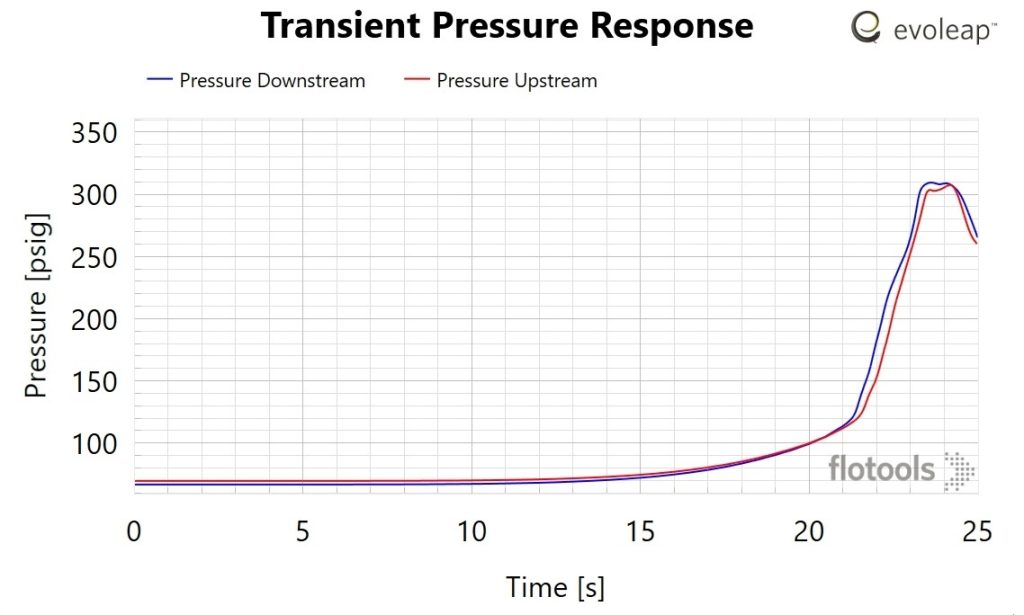
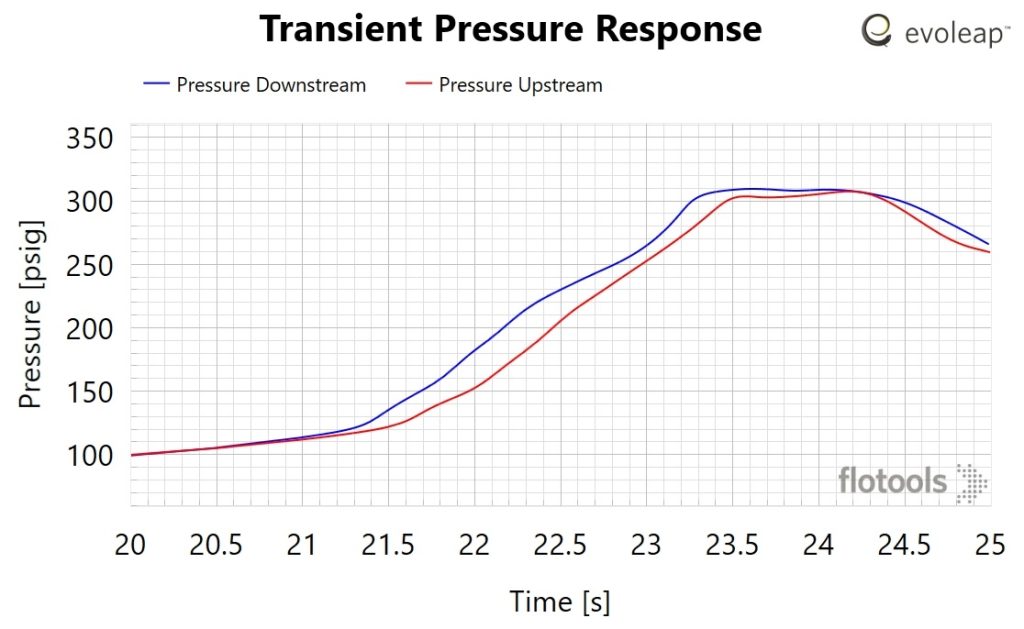
Figure 5 shows the same data but zoomed in on the time when the rapid pressure rises and maximum pressures occur. At 22 s, the upstream and downstream pressures are 153.5 and 183.6 psig, respectively, giving a net force of (183.6 – 154.5) * 672 = 19.6 kips exerted in the upstream direction. Such calculations are performed at every time step for every pipe segment across the entire simulation. The results can be used to compare with rated limits to determine fitness for service. In this case, the Maximum Surge Pressure (MASP) is 440 psig, which is equivalent to 296 kips. Also, the raw results can be exported and used in standard piping analysis software, such as Caesar II. In general, if piping loads exceed limits, possible mitigations are:
- Changes in the closing characteristics of the valves (e.g. faster initially and slower at the end),
- Changes in the valve closure times,
- Reduction of the maximum allowable flow rate,
- Addition of surge relief,
- Addition of surge tanks,
- Shorten segments (e.g. expansion loops),
- Bypasses that divert flow.
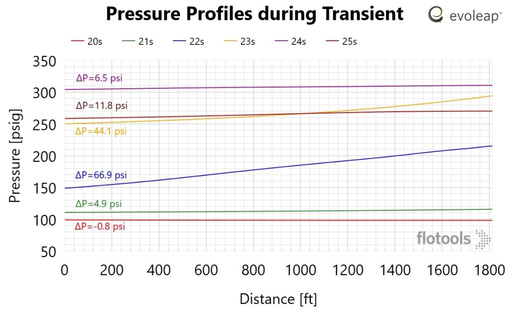
Pressure profiles across the pipe segment at 1 s intervals are shown in Figure 6. The piping load at any time is directly proportional to the difference in pressure across the segment. The maximum piping load depends on the sharpness of the pressure wave (steeper slope), the length of the pipe segment (bigger pressure difference), and the area of the pipe (larger pipes will experience larger loads).
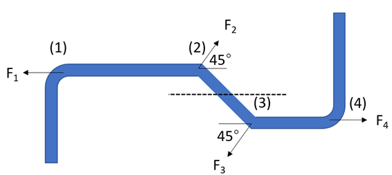
More complicated geometries also require consideration. For example, Figure 7 shows a common configuration with a pair of 45° bends. At a 45° bend, the pressure force is directed at a 45° angle to the pipe axis. Thus, there is a net force, even under steady-state conditions, on the segments 1-2 and 3-4. Under steady state conditions, the sum of forces F1, F2, F3 and F4 are effectively zero. However, as the forces are offset, there is a moment imposed on the system which tends to make the piping system straighten out. This is the same effect that makes a garden hose straighten out when it is pressurized.
Other situations that require special consideration are pipe segments with check valves or valves that may be closed or are actuated in the transient event and pipes with a change in diameter.
For further information, please contact Trent Brown at trent.brown@evoleap.com.