A common flow assurance study objective is calculating the time required to reach hydrate conditions during a shutdown (typically from steady state). This is often referred to as ‘Cooldown’. The ability for an operator to understand the amount of time that is available to safely complete various tasks during a shutdown, or how close to the hydrate region they can operate a pipeline before running into problems is incredibly valuable.
This discussion will cover how one can run large simulation matrices for cooldown efficiently with flotools and will compare the flotools methodology with traditional methods using the OLGA GUI.
Pre-Processing
In flotools, you can setup and create large numbers of cases for a project, and post-process the results quickly. For this case, we are looking for the cooldown times to the hydrate formation temperature for a system with varying parameters: Gas Lift Rate, Flowrate, Inlet Temperature, Water cut, and different fluids. flotools makes this process very simple and easy using the Parametric Studies tool.
With a large case matrix, it can be time-consuming to create all the varying simulations in OLGA. The flotools Parametric Studies tool can create model files by replacing the text of a base file with new parameters. For example, if you have a boundary node with PRESSURE = 100 psig you can give flotools a list of comma-separated values (100, 150, 200) and flotools will create 3 separate key files that are copies of the base file, one with 100 psig, one with 150 psig, and one with 200 psig at that node.
The only inputs needed are the variables to be varied, the parameters for each variable are defined only once. Cases can be named interactively, based on the parameters used.
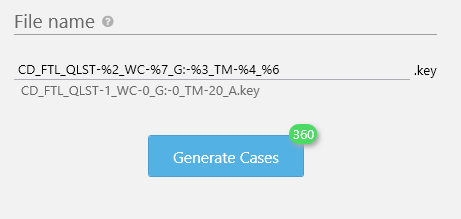
The naming of cases is interactive with the inputs listed above. Each variable has an index associated with it, e.g., WC is associated with %7 (seventh study variable). The index associated with each variable can then be input back into the naming line with the %n operator to have them change with each variation of the parameters. You can even create linked variables that are not used for anything except for naming; for example, the 2nd (%2) and 6th (%6) variables above. Also, the total number of cases to be generated is indicated on the generate cases button with a small green number badge, 360 in this example. This is how many cases we will be generating with these inputs, coming from:
5 flowrates x 3 gas lift rates x 4 temperatures x 2 fluids x 3 water cuts = 360 cases
Once the matrix is set and named appropriately for the parameters of our study, flotools will create the 360 .key files in a location of our choice. flotools can output the .key/model files to any location in the directory structure as well as generate a batch file if necessary. The cases are then ready to run.
Post-processing
Due to the large number of cases, post-processing of the results was time consuming. When using the OLGA GUI to extract simulation results for many cases you are limited by the number of cases that can be load into the GUI simultaneously. For this project, each case output file was relatively small (.tpl and .ppl file size combined to about 2 MB for each case). We were only able to load 47 of the fully completed simulations into the GUI at one time. When extracting trend and profile data you can only take data from those cases loaded into the GUI at a given time. This project required 8 separate extractions to get the full data set, which consumed a lot of extra time to load cases into the OLGA GUI.
Whereas with the flotools route, you can load the cases into a flotools workspace and be ready for plotting immediately.
Both methods are the setup for plotting and tabulating results. In Excel, to create a plot of cooldown times requires some combination of MATCH and INDEX/OFFSET formulas for each series of the MDTHYD output in the case matrix. Following this, the rest of the data must then be formatted in the right way to form a table/pivot table that you can then use to plot based on different parameters.
In flotools, there are built-in calculations for DTHYD and its (MDTHYD, MDPHYD, MAXDTHYD, MAXDPHYD), which can be used without even having to input a hydrate curve in OLGA. Hydrate curves can be input in flotools during post-processing, which flotools will then reference in comparison to the temperatures and pressures over the entire flow path during the simulation.
A comparison of the methods described above are illustrated in the following figure:
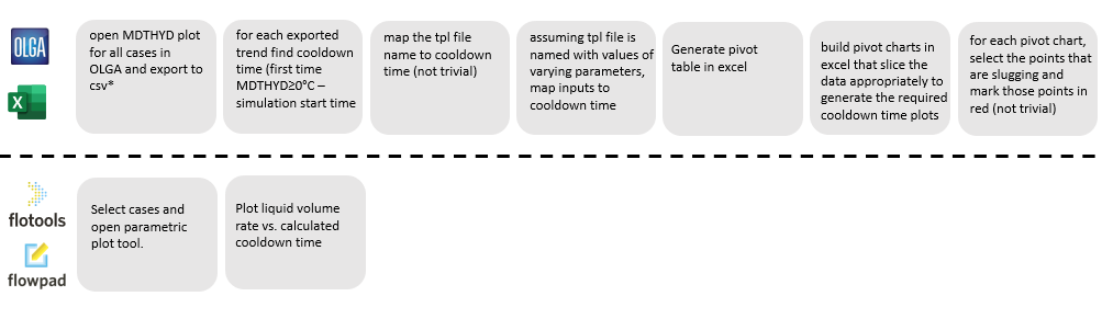
Even for large case matrices, creating all the model files to run is incredibly easy and fast with flotools. Without pre-processing the entire set of cases was created in less than 2 minutes in this instance.
Conversely, post-processing using the OLGA GUI and Excel took roughly 5 times as long to create a finished product of plots or tables. This is mainly due to limitations of the OLGA GUI as to how much info can be stored at one time, i.e., how many cases it can load simultaneously. Having to export the data in chunks was a time-consuming part of the process.
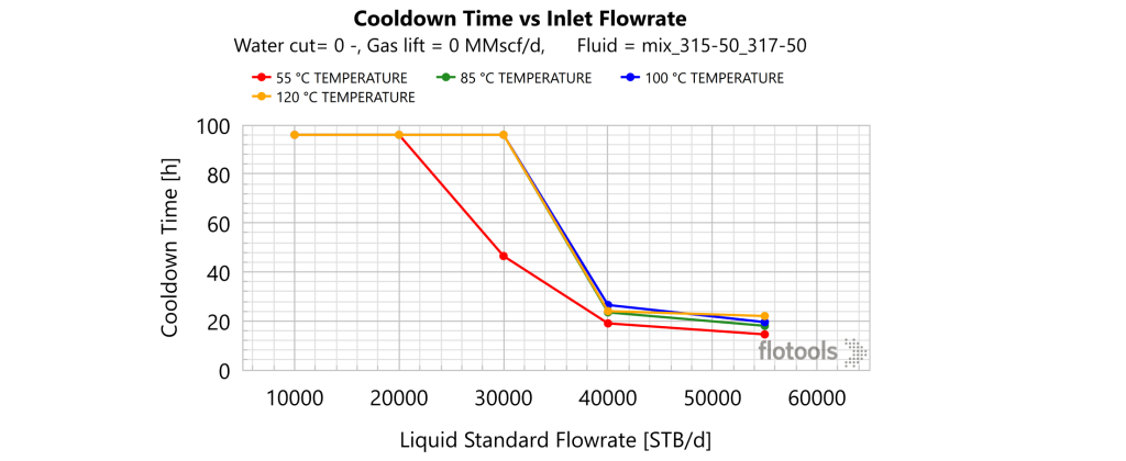
For this set of 360 cases, the goal was to create 11 plots that show the effects of each set of parameters of the parametric study. An example plot created in flotools is show below.
Time breakdowns of each method are given below (these times reflect an experienced user of each method):
OLGA/EXCEL method:
- Open cases in GUI and export MDTHYD to .csv (22 minutes)
- Find first MDTHYD > 0 °C (2 minutes)
- Format all parameters and cooldown times in a table format (5 minutes)
- Create pivot table, slicers, and pivot charts (7 minutes)
- Format plots (create titles, axis labels, etc.) (20 minutes for 11 plots)
- Total (56 minutes)
flotools method:
- Open flotools and load cases (5 minutes)
- Open parametric study tool and select variables and filters/slicers. (2 minutes)
- Change plot formatting to liking (2 minutes)
- Duplicate plot and change filters/slicers (2 minutes for 11 plots)
- Total (11 minutes)
This time difference is especially impactful if the case matrix is updated or if simulations are re-run. If a similar parametric study needs to be run, you can simply copy the parametric study in flotools and modify it instead of having to make a completely new one, whereby saving time on future work.
Conclusion
flotools makes running common flow assurance tasks such as cooldowns easy to create, run and report, even if with many cases. There is a significant time savings with flotools as compared to using the OLGA GUI because flotools can handle all the cases from a project at once and can plot them instantly rather than requiring post-processing in Excel.