Recently, I saw a discussion of OLGA speed in the OLGA Users group on LinkedIn. The discussion starts with the question of why OLGA performs nearly the same on two different CPUs (an Intel Core i7 processer running at 3.4 GHz and Intel Core i5 processor also running at 3.4 GHz). This result is surprising and troubling because Core i5 is a considerably cheaper processor.
I have seen flow assurance companies buy expensive hardware in hope of making OLGA go faster. Unfortunately, the results of such expense have been hit-or-miss. As a budding flow assurance consultant, I witnessed one of those misses. After purchasing hardware that was very expensive, we found that OLGA ran just as fast as it was running on desktop machines that were one year old. Since then, I have spent quite of bit of time looking at OLGA speed and working on understanding what factors impact OLGA performance.
To help flow assurance companies considering such buying decisions, I thought it might be worthwhile sharing the knowledge I have gained through my investigation. Also, I thought it might be interesting to add some data and analysis to the discussion and look specifically at how the number of threads plays a role in OLGA speed. In the LinkedIn discussion, Torgeir Vanvik from Schlumberger offered some excellent insight into the way OLGA works, and I am hoping this post sheds more light on the topic of OLGA’s parallel performance.
Key factors that affect OLGA simulation speed
There are a several key factors that affect OLGA simulation speed. Some have to do with the numerical modeling complexity and others have to do with the hardware on which OLGA is run.
On the modeling side, the most obvious factor is the complexity of the network being modeled. In general, single branch models run faster than networks and simple converging networks run faster than diverging networks or networks with looped lines. Unfortunately, this is not something flow assurance engineers can control so it is not worth discussing it further.
Next on the list are the section lengths and numerical time step. In OLGA, the simulation time step is controlled using the parameters MINDT and MAXDT in the INTEGRATION specification and also using the DTCONTROL parameters. To ensure model stability, simulations are typically run with the CFL condition controlling simulation time step. The CFL condition determines how much distance, relative to the length of a section in the model, the fluid in that section is allowed to move in one time step. The net effect is that the longer the section length, the longer your time steps are allowed to be, and vice versa. The INTEGRATION and DTCONTROL parameters along with section lengths have a profound impact on model speed. The model speed is typically governed by the smallest section in the network. I can write a whole treatise on this but that is a topic for another day.
The model speed is typically governed by the smallest section in the network
On the hardware side, the key factors that affect simulation speed are CPU and I/O speed.
The processor
Modern CPUs have two specifications that are important for our purposes – clock speed and number of cores. The clock speed is indicative of how many instructions are processed per second, and the number of cores indicate how many instructions are processed in parallel. Modern versions of OLGA (6 and above) are able to exploit the power of multiple cores whereas older versions of OLGA (5 and below) get no benefit from multi-core processors.
No matter what the version of OLGA, clock speed is important. Ultimately, it comes down to how many instructions can be processed per second, so the GHz of the processor (the bigger the better) is important.
No matter what the version of OLGA, clock speed is important
For OLGA 6 and later versions, the number of cores will also play a role in the speed. However, it is easy to fall into the trap of believing that more cores will result in faster simulation speeds. The unfortunate reality is that some tasks benefit from being processed in parallel while others don’t. If the time to split the task into small problems is greater than the time savings resulting from parallel processing, the task will actually run slower. In other words, depending on the problem there is a theoretical limit to the gains from parallelization. This is also true for OLGA.
To answer practical questions like, “Is it better to have a 3.4 GHz, 4-core CPU or a 2.4 GHz, 16-core CPU?” requires some investigation into OLGA parallelizability. In fact, we explore that very topic later in this post.
Depending on the problem there is a theoretical limit to the gains from parallelization
I/O
Since OLGA outputs simulation results to the disk as it is running, the speed at which it can write out the results can limit (sometimes severely) the run-time speed. There are two common hardware bottlenecks, the hard drive speed (when OLGA is saving locally) and the network bandwidth (when OLGA is writing to a network drive).
Most commercial-grade desktop computers and laptops ship with mechanical hard-drives that spin at 5400 or 7200 rpm, while server-grade machines often come with 10k or 15k rpm drives. The read/write access speed scales directly with the spin speed of the drive. In general, the greater the spin rate the better the hard drive when it comes to OLGA speed. Solid state drives (SSDs) are now also available cheaply and the technology has matured enough to be used in a commercial setting. However, the speed of SSDs range from worse than mechanical drives to exceptionally fast depending on the manufacturer and model. In other words, not all SSDs are as blazing fast as they would have you believe so choose carefully. It is also important to consider the computer bus interface which determines the internal data transfer rates (though these days that interface is rarely the bottle neck). Ultimately, the hard drive performance can be as important to simulation speed as the CPU.
Ultimately, the hard drive performance can be as important to simulation speed as the CPU
When saving OLGA results to a network share, the network can also limit the ability for OLGA to write simulations results. As a result, companies should ensure that the bandwidth between the computer running OLGA and the network storage is as large as possible. This will alleviate any slowdowns in OLGA speed.
When saving OLGA results to a network share, the network can also limit the ability for OLGA to write simulations results
These bottlenecks can also be avoided most of the times by carefully considering the frequency and quantity of simulation outputs.
The study
In order to understand the factors that influence parallel speedup, we used 8 different model configurations.
Model
Description
Number of sections
Smallest section length (m)
1
Single pipeline model
190
173
2
Single branch – fine mesh
7000
11
3
Single branch – coarse mesh
376
21
4
Converging pipeline network
335
17
5
Converging network with pressure-pressure boundary
383
14
6
Converging pipeline network – no flow
335
17
7
Converging-diverging network (Loop)
60
50
8
Two separate networks
426
50
Methodology
All models were run with no trend and profile outputs to eliminate the effect of I/O on parallel speedup. To ensure the results we repeatable, each model was run multiple times utilizing a varying number of threads. A simple program was developed to run each model up to 20 times in 10 minutes (which ensured all models ran at least 2 times and many ran the full 20 times). The average run time was then calculated for each model and thread combination. It is worth noting that the run times for each simulation iteration were nearly identical. OLGA 2014.2 was used for this study (see acknowledgments at the end). The following command was used to manipulate the number of threads used by OLGA. A thread is a part of a computer program that can be managed separately by the operating system. A single core in a modern CPU can handle two threads.
opi.exe /t <num_threads> <input_file>
All simulations were run on a machine with 4 physical cores and capable of running 8 threads in parallel.
Results
The first plot shows the speedup achieved by the various models. The ideal speedup line shows that a model using n threads should be able to achieve a speedup of ‘n’ compared to the 1 thread model. Note that without specifying the number of cores when running OLGA, the default number of threads is based on the number of CPU cores (in our case that is 4).
Speed-up achieved by various model types
The plot above shows that the best performing model achieves a speedup of 3 using 4 threads, and a speedup of 4 using 8 threads. The worst performing models cap off at a speedup of ~1.6 and achieve no additional speedup beyond 5 threads. In fact, speedup of few of the models reduce when going from 7 threads to 8. However, this last artifact could be a result of using all available threads on the processor leaving the OS to switch between the computational load and background services running on the OS. We can only confirm this if we ran the test on an 8- or 16-core machine.
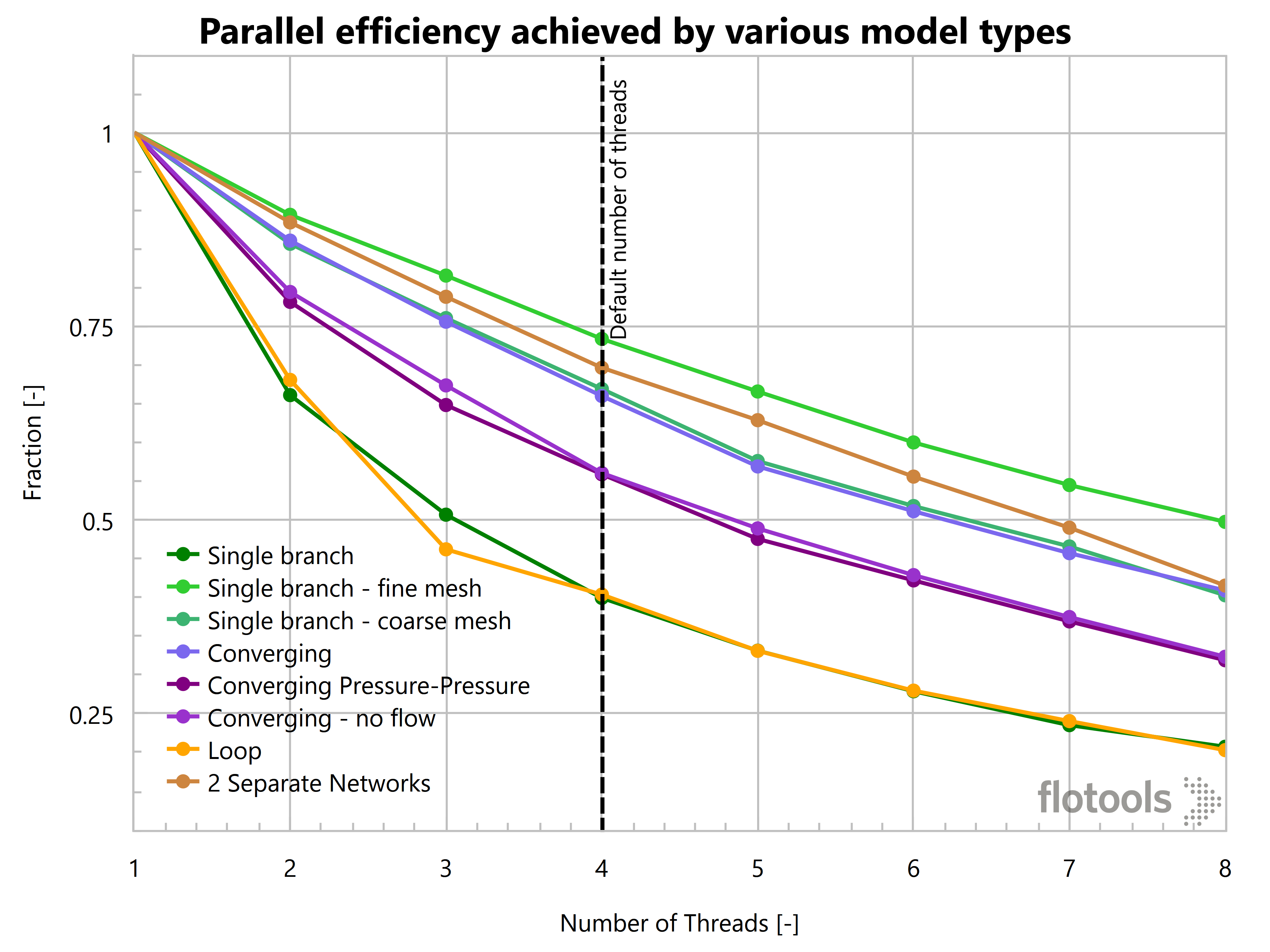
Another way to look at speedup is to look at a quantity called parallel efficiency which is the ratio of the actual speedup to the ideal speedup.
Parallel efficiency achieved by various model types
These two plots show that the parallel speedup tends to stagnate beyond 4 threads for most models. Most models are able to achieve a speedup of 2 or more when using 4 threads. However, by the time we get to 7 threads, only one model has a parallel efficiency of over 50%. In other words, we would be better off running two simulations simultaneously using 4 threads each, rather than running just one simulation using all 8 available threads.
Parallel speedup tends to stagnate beyond 4 threads for most models
Analysis
The parallel speedup and efficiency plots showed that the efficiency of parallelization varied between various model types. So the next question is what makes a model more or less parallelizable. The flow chart below shows a simplified program structure of a parallel program.
Typical program flow of a parallel numerical algorithm such as the one used in OLGA
In OLGA, the main calculation loop would be the time loop that marches time from start to the end of the simulation. The initial sequential process would be reading input files, tab files, etc. The final post-processing might include closing file handles, releasing memory, etc.
With that background in mind, we curve fitted the parallel efficiency curves with an exponential function of the following form:
where
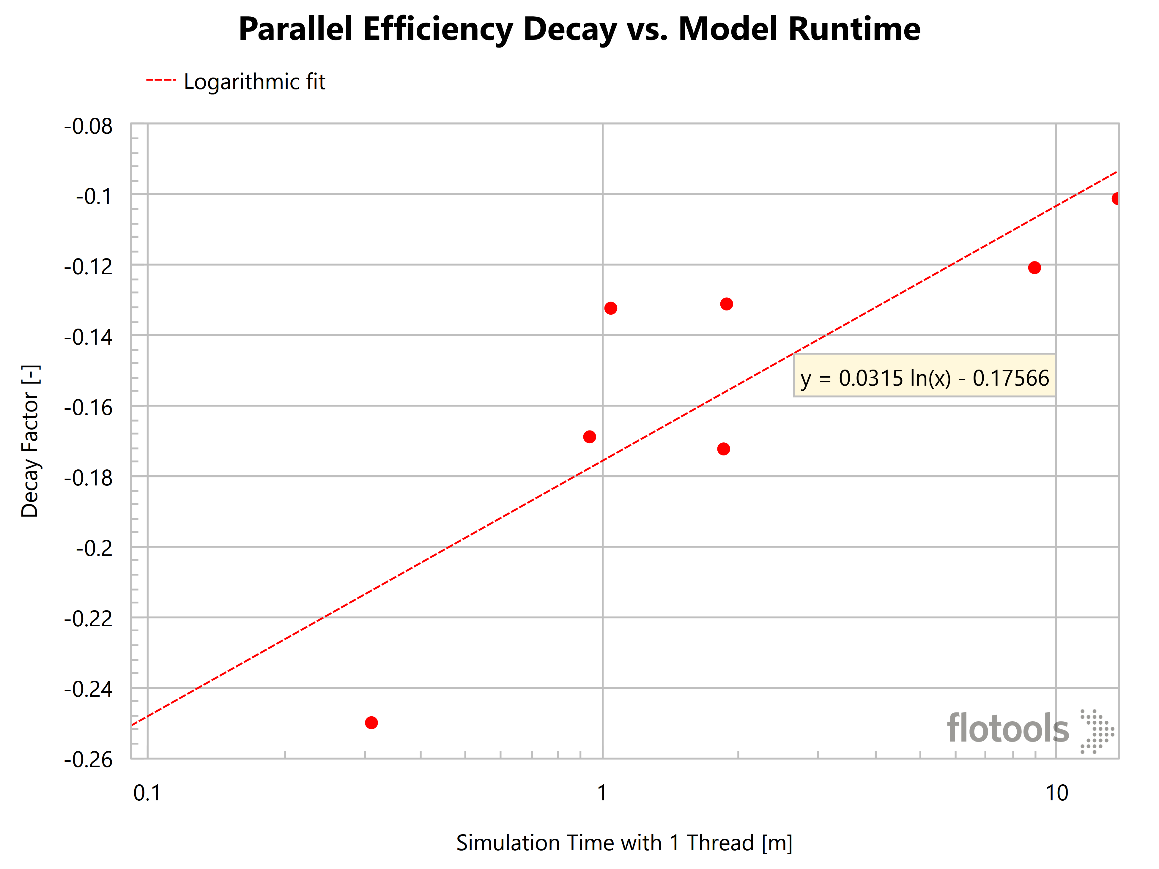
I call the calculated factor the parallel efficiency decay factor. We can then plot the decay factor as a function of various aspects of the model. Our analysis shows that the decay factor is a strong function of the model runtime and the number of sections in the model.
Parallel Efficiency Decay vs. Model Runtime
The plot above shows that the parallel efficiency is loosely a logarithmic function of the model run time. This makes sense and follows readily from the way parallel efficiency is formulated above. (and Amdahl’s law). Skipping some math jugglery, can be rearranged to the following equation:
where
When , there is hardly any speedup, yielding a parallel efficiency of and when , yielding a parallel efficiency of 1. In between, we get a log-linear relationship.
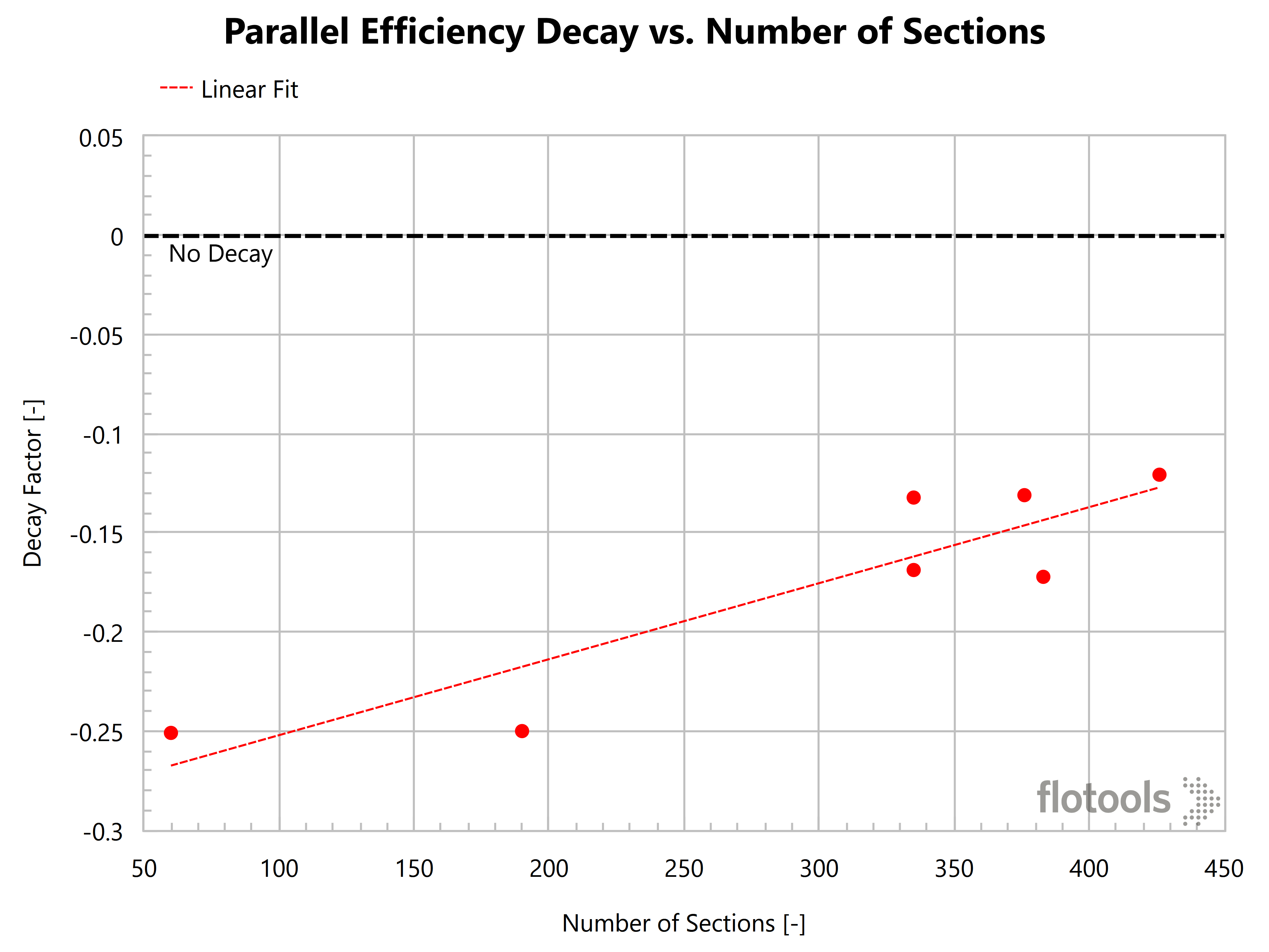
The plot below shows the parallel efficiency decay factor as a function of number of sections in the model. As the number of sections increase, parallel efficiency gets better. Note that at 7000 sections, the decay factor is ~-0.1, which is probably close to the theoretical limit based on the strictly sequential parts of the simulation.
Parallel Efficiency Decay vs. Number of Sections
This also makes sense based on the fact that the number of computations performed in each time step is directly proportional to the number of sections and these are the computations that are computed in parallel according to the OLGA manual. So, higher the number of sections, better the parallel efficiency. However, there is a limit to the parallel efficiency as there are always sequential parts of the algorithm that cannot be parallelized.
Higher the number of sections, better the parallel efficiency
To sum it up…
Getting back to the discussion of hardware choices and their impact on OLGA speed, number of cores, clock speed and I/O speed are all significant factors. Recent versions of OLGA are multi-threaded and have the ability to run faster by utilizing multiple processor cores. We did a detailed analysis on how number of cores can impact OLGA speed and whether it is prudent to spend money on cores.
OLGA defaults to using as many threads as the number of cores available. In our analysis, the best speedup we achieved with 4 threads was ~3, a 75% parallel efficiency. In general, the more compute intensive the simulation, the better the speedup. For short simulations, multi-threading did not help. Even for a long simulation with 7000 sections, going from 4 threads to 8 threads only bumped up the speedup from 3 to 4. In general the parallel efficiency tapers off as we go beyond 4 threads. Based on our analysis, I reckon that 4 threads is a sweet spot for running flow assurance models in OLGA. You could of course fiddle with this for individual models but I would not recommend spending time on it.
Four threads is a sweet spot for running flow assurance models in OLGA
Keeping in line with our findings, the OLGA manual advises that it is better to use the available cores for simultaneous simulations rather than using them to speed up an individual simulation. However, this advice is a bit naive. For example, most professional desktop or laptop systems today have 4 cores but do not have the hard drive access speeds to support 4 simultaneous simulations writing data. The right choice lies somewhere in the middle.
If you are making a hardware buying decision I would not go beyond 4 cores when buying a computer with a mechanical hard drive. If you have enough OLGA licenses and want to centralize your simulations on one machine, the storage choice is as important as the processor choice. I would also recommend setting OMP_NUM_THREADS environment variable to 4 in order to run OLGA at an optimum parallel efficiency.
We welcome you to share your experiences and provide us feedback. If there is enough interest, we will explore the effect of CPU clock speed and disk I/O in detail in future posts.
Acknowledgments
We thank Dr. Ivor Ellul and RPS Group for running OLGA simulations and for valuable suggestions related to the analysis presented here.
5 thoughts on “The Truth about OLGA Speed”
Abhinav Priyadarshi says:
Very detailed and informative analysis. Thanks for doing this.
I had few queries:
1) When you say older versions of OLGA (5 and older) have no benefits of multi-core processing, you mean that they use only single – core? So all that matters for OLGA (5 and older) is writing speed I/O and clock time?
2)When you set OMP_NUM_THREADS environment variable to 4 in order to run OLGA at an optimum parallel efficiency then even if you run 2 independent simulations in parallel will the core use be still limited to 4, even if the machine is 8 core processor?
When you say older versions of OLGA (5 and older) have no benefits of multi-core processing, you mean that they use only single – core? So all that matters for OLGA (5 and older) is writing speed I/O and clock time?
Yes all versions of OLGA prior to OLGA 6 are single threaded. So yes the major factors are clock speed of CPU and the I/O speed.
When you set OMP_NUM_THREADS environment variable to 4 in order to run OLGA at an optimum parallel efficiency then even if you run 2 independent simulations in parallel will the core use be still limited to 4, even if the machine is 8 core processor?
Each of the simulations will use the number of threads specified in OMP_NUM_THREADS. So if you started two simulations you would be utilizing 8 threads. For an 8 core hyper-threaded CPU, you can run up to 4 simulations (each utilizing 4 threads for a total of 16 threads). Please bear in mind if you run too many simulations on the same machine I/O speed can easily become the bottleneck.
Thanks for the detailed analysis. I have a few comments/discussion points:
1. I feel that these results might be a bit hardware dependant.
It looks to me like you used a 4 core processor with Hyper-threading which is a feature of some of the high end Intel processors. From what I understand this assigns two virtual (or logical) cores to each physical core of the processor (giving 8 virtual cores). The idea behind this is to increase the utilisation of each core, as there are two logical processors, with one using the processor resources whilst the other is stalled. Essentially this makes more efficient use of the processor resources, as it allows a second thread to be run in any ‘downtime’ in the first thread. The end result of this is that you should expect diminishing returns when increasing the number of threads beyond the number of physical cores of your CPU. That’s why I don’t think it’s a coincidence that you found 4 cores to be the optimum in efficiency!
As you’ve shown, the nature of the software is such that it doesn’t scale perfectly with the number of threads used. However, assuming we had a program that did scale perfectly on the software side, you should still expect to see worse performance scaling beyond 4 threads, as a situation would then arise in which each physical core would start sharing resources between 2 threads.
For the same reasons:
a) don’t expect to get the same performance when running two simultaneous simulations with 4 threads.
b) if running an older version of OLGA which doesn’t use multi-threading, disable hyper-threading on the PC if you can.
I feel some additional analysis with a different processor would give better insight into whether 4 threads is actually the optimum when it comes to OLGA’s performance scaling with multi-threading. There are Intel processors available with 6 or 8 physical cores (12 or 16 logical cores respectively with hyper-threading), so I would be interested to see if the ‘sweet spot’ is actually at the number of physical cores available.
2. Hardware is cheaper than software
Although 4 threads on your machine appears to be a ‘sweet spot’, there’s still absolute gains in performance at higher numbers of threads. Therefore it would be better to have a dedicated PC for each licence you have and use the maximum number of threads available (or maybe a couple less given that some of your results showed no improvement going from 7 to 8 threads) – considering the high cost of software licences, hardware is relatively cheap and it makes sense to use each licence as efficiently as possible.
3. If you want to reduce the possibility of I/O bottlenecks:
Try a RAM Disk – Google that one (that might be a bit extreme though).
James, thanks for your comment. We did have the same questions that you pose in your first comment when we did the study. So we are planning to extend the study to machines with 8 and 16 physical cores. I have mixed feelings about comment #2 and #3. While theoretically what you are saying makes sense, in a practical setting there are some other considerations.
Typically your IT department wants to reduce and consolidate the resources they are managing. If you have 8 licenses, they don’t want to 8 machines that they have to worry about failures, software updates, security patches, etc.
If you combine all the features that we are discussing (8- or 16-core CPU, SSD/Flash Disk), we could start getting into the range where hardware costs are substantial as compared to the software maintenance cost
Another possible direction, which at least a couple of our customers are exploring, is moving compute instances to the cloud (like AWS EC2) and there the choice of hardware makes a big difference in your monthly costs.
All said, I do appreciate you reading the article and thinking deeply about the issue. We hope to follow up with some more information on this subject in the coming weeks and months.

 Recently, I saw a discussion of OLGA speed in the OLGA Users group on LinkedIn. The discussion starts with the question of why OLGA performs nearly the same on two different CPUs (an Intel Core i7 processer running at 3.4 GHz and Intel Core i5 processor also running at 3.4 GHz). This result is surprising and troubling because Core i5 is a considerably cheaper processor.
I have seen flow assurance companies buy expensive hardware in hope of making OLGA go faster. Unfortunately, the results of such expense have been hit-or-miss. As a budding flow assurance consultant, I witnessed one of those misses. After purchasing hardware that was very expensive, we found that OLGA ran just as fast as it was running on desktop machines that were one year old. Since then, I have spent quite of bit of time looking at OLGA speed and working on understanding what factors impact OLGA performance.
To help flow assurance companies considering such buying decisions, I thought it might be worthwhile sharing the knowledge I have gained through my investigation. Also, I thought it might be interesting to add some data and analysis to the discussion and look specifically at how the number of threads plays a role in OLGA speed. In the LinkedIn discussion, Torgeir Vanvik from Schlumberger offered some excellent insight into the way OLGA works, and I am hoping this post sheds more light on the topic of OLGA’s parallel performance.
Recently, I saw a discussion of OLGA speed in the OLGA Users group on LinkedIn. The discussion starts with the question of why OLGA performs nearly the same on two different CPUs (an Intel Core i7 processer running at 3.4 GHz and Intel Core i5 processor also running at 3.4 GHz). This result is surprising and troubling because Core i5 is a considerably cheaper processor.
I have seen flow assurance companies buy expensive hardware in hope of making OLGA go faster. Unfortunately, the results of such expense have been hit-or-miss. As a budding flow assurance consultant, I witnessed one of those misses. After purchasing hardware that was very expensive, we found that OLGA ran just as fast as it was running on desktop machines that were one year old. Since then, I have spent quite of bit of time looking at OLGA speed and working on understanding what factors impact OLGA performance.
To help flow assurance companies considering such buying decisions, I thought it might be worthwhile sharing the knowledge I have gained through my investigation. Also, I thought it might be interesting to add some data and analysis to the discussion and look specifically at how the number of threads plays a role in OLGA speed. In the LinkedIn discussion, Torgeir Vanvik from Schlumberger offered some excellent insight into the way OLGA works, and I am hoping this post sheds more light on the topic of OLGA’s parallel performance.


%7D) where
where
 I call the calculated
  factor the parallel efficiency decay factor. We can then plot the decay factor as a function of various aspects of the model. Our analysis shows that the decay factor is a strong function of the model runtime and the number of sections in the model.
%7D%7Bn_p-1%7D) where
where
 When
When  , there is hardly any speedup, yielding a parallel efficiency of
  and when
  ,
,  yielding a parallel efficiency of 1. In between, we get a log-linear relationship.
The plot below shows the parallel efficiency decay factor as a function of number of sections in the model. As the number of sections increase, parallel efficiency gets better. Note that at 7000 sections, the decay factor is ~-0.1, which is probably close to the theoretical limit based on the strictly sequential parts of the simulation.
yielding a parallel efficiency of 1. In between, we get a log-linear relationship.
The plot below shows the parallel efficiency decay factor as a function of number of sections in the model. As the number of sections increase, parallel efficiency gets better. Note that at 7000 sections, the decay factor is ~-0.1, which is probably close to the theoretical limit based on the strictly sequential parts of the simulation.
Very detailed and informative analysis. Thanks for doing this.
I had few queries:
1) When you say older versions of OLGA (5 and older) have no benefits of multi-core processing, you mean that they use only single – core? So all that matters for OLGA (5 and older) is writing speed I/O and clock time?
2)When you set OMP_NUM_THREADS environment variable to 4 in order to run OLGA at an optimum parallel efficiency then even if you run 2 independent simulations in parallel will the core use be still limited to 4, even if the machine is 8 core processor?
Thanks
Abhinav
Yes all versions of OLGA prior to OLGA 6 are single threaded. So yes the major factors are clock speed of CPU and the I/O speed.
Each of the simulations will use the number of threads specified in OMP_NUM_THREADS. So if you started two simulations you would be utilizing 8 threads. For an 8 core hyper-threaded CPU, you can run up to 4 simulations (each utilizing 4 threads for a total of 16 threads). Please bear in mind if you run too many simulations on the same machine I/O speed can easily become the bottleneck.
Thanks Michael
Thanks for the detailed analysis. I have a few comments/discussion points:
1. I feel that these results might be a bit hardware dependant.
It looks to me like you used a 4 core processor with Hyper-threading which is a feature of some of the high end Intel processors. From what I understand this assigns two virtual (or logical) cores to each physical core of the processor (giving 8 virtual cores). The idea behind this is to increase the utilisation of each core, as there are two logical processors, with one using the processor resources whilst the other is stalled. Essentially this makes more efficient use of the processor resources, as it allows a second thread to be run in any ‘downtime’ in the first thread. The end result of this is that you should expect diminishing returns when increasing the number of threads beyond the number of physical cores of your CPU. That’s why I don’t think it’s a coincidence that you found 4 cores to be the optimum in efficiency!
As you’ve shown, the nature of the software is such that it doesn’t scale perfectly with the number of threads used. However, assuming we had a program that did scale perfectly on the software side, you should still expect to see worse performance scaling beyond 4 threads, as a situation would then arise in which each physical core would start sharing resources between 2 threads.
For the same reasons:
a) don’t expect to get the same performance when running two simultaneous simulations with 4 threads.
b) if running an older version of OLGA which doesn’t use multi-threading, disable hyper-threading on the PC if you can.
I feel some additional analysis with a different processor would give better insight into whether 4 threads is actually the optimum when it comes to OLGA’s performance scaling with multi-threading. There are Intel processors available with 6 or 8 physical cores (12 or 16 logical cores respectively with hyper-threading), so I would be interested to see if the ‘sweet spot’ is actually at the number of physical cores available.
2. Hardware is cheaper than software
Although 4 threads on your machine appears to be a ‘sweet spot’, there’s still absolute gains in performance at higher numbers of threads. Therefore it would be better to have a dedicated PC for each licence you have and use the maximum number of threads available (or maybe a couple less given that some of your results showed no improvement going from 7 to 8 threads) – considering the high cost of software licences, hardware is relatively cheap and it makes sense to use each licence as efficiently as possible.
3. If you want to reduce the possibility of I/O bottlenecks:
Try a RAM Disk – Google that one (that might be a bit extreme though).
Let me know your thoughts!
Regards,
James
James, thanks for your comment. We did have the same questions that you pose in your first comment when we did the study. So we are planning to extend the study to machines with 8 and 16 physical cores. I have mixed feelings about comment #2 and #3. While theoretically what you are saying makes sense, in a practical setting there are some other considerations.
All said, I do appreciate you reading the article and thinking deeply about the issue. We hope to follow up with some more information on this subject in the coming weeks and months.
Cheers!